

In my last post, I began explaining the math behind power structure theory (PST). For context, a power structure is a system of relationships among political actors with varying levels of strength. Power structures can be found in a wide variety of settings, such as the international system, national politics, and within organizations — basically anywhere people are struggling for political power.
In Part 1, I explained the law of motion, which describes how power flows around the network of a power structure, making some actors stronger and others weaker. In this post, I’m going to explain the two other equations at the heart of power structure theory: the utility function and PrinceRank.
Whereas the law of motion describes how the power levels of the actors change as a result of their relationships with each other, these two equations describe the converse process: how actors change their relationships as a result of the structure itself. The back and forth between these two processes — changes in power and changes in relationships — is what gives rise to some of the dynamic phenomena that we see in power politics.
I went out of my way in Part 1 to slow walk readers through the math underlying the law of motion — primarily because it uses matrices, which are unfamiliar to many people. The equations in this post are simpler, involving just basic arithmetic and summation. So the focus here will be on what these equations mean rather than how the calculations work.
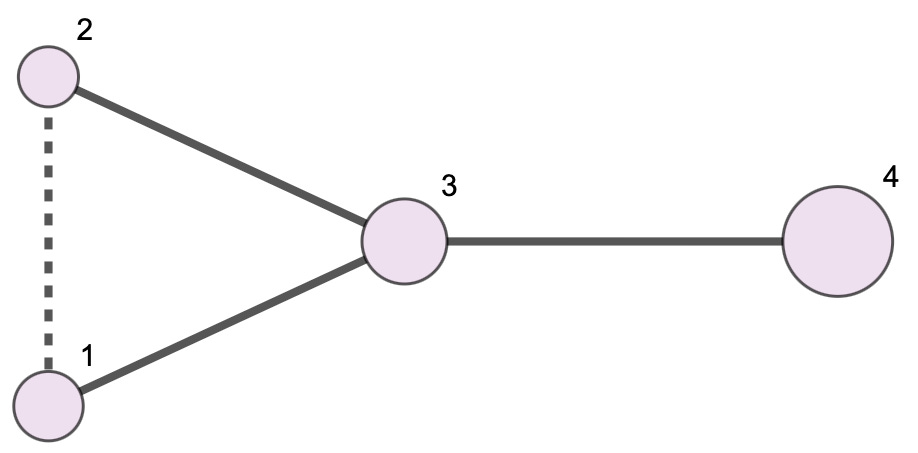
One component of a power structure is a size vector, s, which is a list of numbers indicating how strong the actors are relative to each other. The size vector represents the distribution of power in the system.

A second component of a power structure is a tactic matrix which describes the relationships among the actors, or how they’re using the power that they have. Within this abstraction, the actors’ scope of action is confined to altering their relationships with each other. That’s all they can do: choose where they are on the friend-foe spectrum with respect to every other actor.
To figure out which relationships make sense for each actor and which ones don’t, we first need a theory of what the actors want. That’s what these two equations model.
The Utility Function
Actors in a power structure want one thing: power. The whole “game” is to use the power at one’s disposal to acquire more of it or, on a bad day, just to survive.
But there are two ways that we can think about the acquisition of power. The first is in terms of absolute power. This is not absolute power in the sense of Louis XIV (or Donald XIV for that matter). It means gaining power in absolute terms, or getting more of it today than you had yesterday. Pursuing absolute power means that your size value in s increases.
The other motivation that an actor can have is to pursue relative power. When you pursue relative power, you’re concerned with how much you have relative to other actors, and in general you want more of it than they have. You might even be willing to have less power in absolute terms if it means that your share relative to your competitors increases.
Actors in a power structure want a combination of absolute and relative power, and their preferences lie along a spectrum between those two extremes. In PST, this preference is expressed as a parameter called alpha, or α, which ranges from 2 to 3. Alpha values closer to 2 express a preference for relative power; those closer to 3 represent a preference for absolute power.
The utility function describes how actors “feel” about the distribution of power, given their alpha preferences:
This equation states that an actor’s utility is their size raised to their alpha value, divided by the sum of the squares of all actors’ sizes.1
In general, the utility function says that actors prefer to have absolute power — to be larger rather than smaller, all else being equal. It also implies that actors want to maximize their “market share” of power — that is, to have a greater percentage of the overall total, which means more relative power.
An actor’s utility also increases when its competitors are small and divided rather than united. For example, in the image below there are two distributions of power. In each, one of the actors is highlighted in red. Which of the two distributions is preferable to this actor?
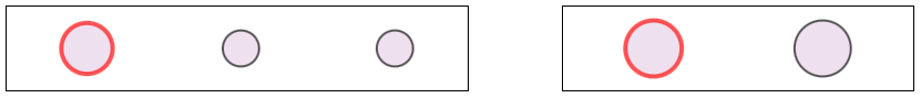
In both of these distributions, the highlighted actor has 50% of the market share of power. However, the utility function says that the distribution on the left is preferable because it entails two competitors with 25% of the power each, rather than a single competitor with 50%. In general, an actor’s utility increases when rival power is dispersed instead of concentrated.
The preferences that I just described are robust in the sense that actors will generally make the same choices regardless of whether they prefer absolute versus relative power. But other trade-offs are more subtle. For example, consider two actors that are equal in size. An actor preferring relative power (α=2) would actually agree to be reduced to 90% of its original size if it meant that the other actor would be reduced more, say to 85%, because then it could dominate. In contrast, an actor preferring absolute power (α=3) would not make that choice: they would rather have an equal-sized peer than suffer a reduction in absolute terms. The utility function encodes these trade-offs.
PrinceRank
The third equation of power structure theory is called PrinceRank. The name is an homage to Machiavelli’s The Prince and Google’s PageRank algorithm. PrinceRank defines a network centrality metric that takes into account negative graph edges (i.e. those representing antagonism). It produces a number that tells us how “happy” each actor is with its place in a power structure. This number is based upon the distribution of power, the relationships among all of the actors, and the actors’ alpha preferences — in other words, the entire abstract power structure object.
The PrinceRank equation is commonly used in economic modeling and game theory to determine intertemporal utility — that is, utility calculated across multiple time steps. Unlike the equations for the law of motion and utility, which took me months of labor to devise, PrinceRank is an equation that I appropriated from the academic literature, applied to this model, and renamed. It is:
The idea here is to take a power structure and run the law of motion iteratively upon it, as in the animation below:
At each time step — i.e. each frame in the animation — PrinceRank takes the utility value of each actor. It then sums up each actor’s utility across time, over the course of the whole animation.2 However, these utility values are not all weighted equally. The ones closer to the beginning of the animation count more, whereas the ones farther into the future count less. This discounting reflects the idea that short-term rewards tend to be more important than long-term ones.
PrinceRank thereby introduces an additional variable into power structure theory. The parameter delta, or δ, determines how heavily future rewards are weighted. Actors with delta values closer to 1 are more concerned about the future; those closer to 0 are more focused the short term. We can think of this as quantifying each actor’s level of patience. So the “personality” of every actor is determined by a combination of their preference for absolute versus relative gains and their level of patience. PST suggests that these are two fundamental characteristics of political actors.
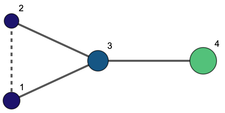
It is convenient to show each actor’s PrinceRank by coloring the nodes in a power structure diagram. I typically use a blue-green spectrum in which blue represents the actors with the lowest PrinceRank (the unhappiest ones) and light green represents the highest, as in the diagram below. Here actor 4 is in the best position, at least initially:
One last observation is that PrinceRank takes into account the entire structure. This means that an actor’s PrinceRank can change even if they don’t alter any of their immediate relationships. Changes in another part of the graph, even several degrees of separation away, can make a difference. Everyone’s fates are interconnected in the fabric of a power structure, and PrinceRank captures that.
Wrap Up
What can we do with this model? One interesting application is that PrinceRank gives us a way to compare different configurations of a particular power structure in order to understand what “foreign policies” the actors might choose. It lets us see whether the actors have incentives to change any of their relationships with each other, and therefore it can illuminate how ongoing interaction among them might unfold.
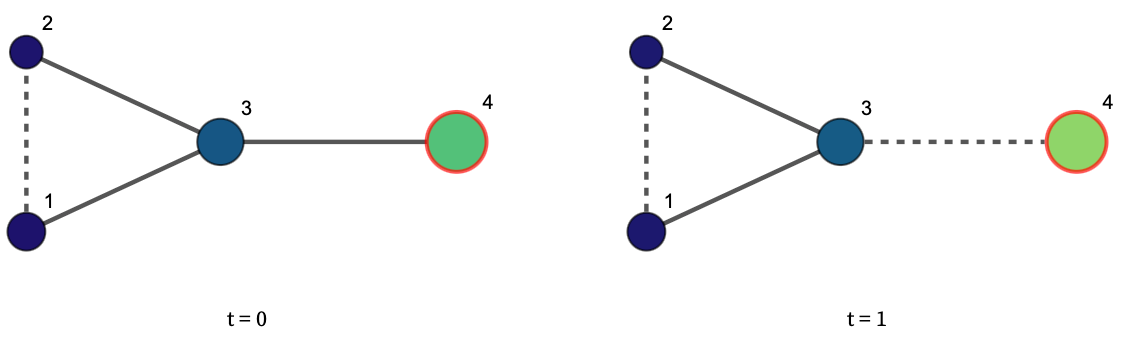
For instance, the figure below shows the same power structure at two different points in time, t=0 and t=1. The highlighted actor has an incentive to attack actor 3 — as indicated by the bright green PrinceRank on the right compared to the darker green on the left. In this example, actor 4 prefers relative gains to absolute ones, and it wants to reduce actor 3 before it becomes more of a threat.
Scaling up this technique, we can “game out” permutations of “moves” based upon techniques similar to those used in chess engines. A game engine in this context would explore a large tree of possible moves and countermoves, searching for the lines of play that result from all of the actors trying to maximize their individual PrinceRanks. The phenomena that emerge from these simulations can express real world power dynamics such as hierarchy formation, balances of power, domination, resistance, revolution, and divide and rule patterns.
Since PST provides a description of how power works, and power is relevant in so many social and historical contexts, this abstraction has wide ranging implications. If you want to learn more, a good place to start is my book, Power Structures in International Politics. To understand how PST can unify neorealism and neoliberalism in international relations, read this.
Technically, u, s, and α are all vectors and everyone’s utility is computed in a single operation.
The infinity symbol in the PrinceRank equation suggests that this summation process goes on forever. However, for practical purposes, the results tend to converge within a few dozen time steps.